Stochastic,model,predictive,braking,control,for,heavy-duty,commercial,vehicles,during,uncertain,brake,pressure,and,road,profile,conditions

Ryota Nakahara·Kazuma Sekiguchi·Kenichiro Nonaka·Masahiro Takasugi·Hiroki Hasebe·Kenichi Matsubara

Abstract When heavy-duty commercial vehicles(HDCVs)must engage in emergency braking，uncertain conditions such as the brake pressure and road profile variations will inevitably affect braking control. To minimize these uncertainties， we propose a combined longitudinal and lateral controller method based on stochastic model predictive control(SMPC)that is achieved via Chebyshev-Cantelli inequality.In our method，SMPC calculates braking control inputs based on a finite time prediction that is achieved by solving stochastic programming elements，including chance constraints.To accomplish this，SMPC explicitly describes the probabilistic uncertainties to be used when designing a robust control strategy.The main contribution of this paper is the proposal of a braking control formulation that is robust against probabilistic friction circle uncertainty effects.More specifically， the use of Chebyshev-Cantelli inequality suppresses road profile influences， which have characteristics that are different from the Gaussian distribution，thereby improving both braking robustness and control performance against statistical disturbances.Additionally，since the Kalman filtering(KF)algorithm is used to obtain the expectation and covariance used for calculating deterministic transformed chance constraints，the SMPC is reformulated as a KF embedded deterministic MPC.Herein，the effectiveness of our proposed method is verified via a MATLAB/Simulink and TruckSim co-simulation.

Keywords Heavy-duty commercial vehicle·Brake system·Stochastic model predictive control·Road profile

Advanced vehicle control features， including traction control， anti-lock braking systems， electronic stability control，adaptive cruise control， lane-keeping assistance， etc.， have been topics of intense study over many years，and a variety of such functions have already been implemented to assist drivers. These and even more advanced driving automation functions are currently being readied for application to passenger cars，buses，and large vehicles whose handling requires superior driving skills. In particular， in emergency situations， advanced braking control is required to regulate the vertical vehicle control of vehicles of buses or trucks with large inertia and bring them to safe stops.Today，most buses and trucks are equipped with pneumatic braking systems that use compressed air as their energy medium.However，pneumatic braking systems have characteristics that make control design difficult[1-4].First，large time delays occur due to the compressibility of air，and the dynamics of pneumatic braking systems inevitably mean that the relationship between the air medium and pressure flow is non-linear. Hence，when combined with the vehicle’s longitudinal dynamics，pneumatic braking systems are prone to various uncertainties. These include supply pressure variations due to brake application and release，temperature increases resulting from frequent braking，brake system component wear，vehicle load fluctuations， and changes in road surface conditions due to rain or snow.

When considering such factors，model predictive control(MPC) [5]， which considers dynamic coupling [6，7]， topographical information[8]，and horizontal vehicle dynamics，provides an optimal control method for safe vehicle control during emergency stop conditions.For that reason，MPC is incorporated into a wide variety of automatic control systems such as train pneumatic braking systems [9]， bus braking energy efficiency systems[10]，and the steering systems of all-terrain cranes with slow dynamic response levels [11].The high utility of MPC is its ability to solve the constrained optimization problem of a finite-time interval for each sampling step based on the model to be controlled.Then the controller applies the first component of the calculated input series in each sampling step. MPC makes it possible to calculate control inputs that explicitly consider functional，physical，and safety restrictions by applying constraints for input and state.However，MPC is vulnerable to the influence of actual motion factors that are not considered in models. Therefore， although preset constraints may be satisfied in MPC predictions， those constraints may be exceeded in actual conditions. MPC-based control has also been applied to heavy-duty commercial vehicle (HDCV)wheel slip control [12，13]， fuel consumption systems [14-17]，automatic hydraulic transmission systems[18]，actuator time delay controllers [19]， pneumatic actuator controllers[20]. The challenge of the controller design of HDCVs are robustness against model uncertainty due to actuator or loading.The methods proposed in[21]is not considered against the uncertainty of the plant model. Also， the Kalman filer(KF) embedded MPC brake system [22] is available to use state covariance for the controller.To solve that，robust antislip control systems for different road surface environments[23] and systems that compensate for vehicle specification changes caused by load variations[24，25]is reported.However，the deterministic constraints result in aggressive inputs when the model has stochastic uncertainty.This may result in the model not complying with the constraints as theory suggests.

In contrast， stochastic model predictive control (SMPC)is a robust control method that considers such uncertainties.In the SMPC approach，which is shown in Fig.1，we can see that SMPC inputs a stochastic constraint called a “chance constraint”based on the probability distribution of the prediction error and designates it as the upper and lower limits of the state.This allows SMPC to explicitly describe the probabilistic uncertainties in designing the robust control strategy.For example， let the deterministic constraint bex≤xmax，withxas the states andxmaxas the upper limit states. Ifxis uncertain， the probability will not reach fifty percent. To avoid creating too large a value，the deterministic constraint needs to converted into a probabilistic (also called chance)constraint，in which Pr(x≤xmax)≥1-α，withα∈(0，0.5]is the allowable probability. In many applications， system uncertainties are often considered to be stochastic processes，which allows the incompleteness and uncertainties of set optimization problems to be taken into consideration. This suppresses erroneous control that can result from discrepancies between theory and an actual environment. SMPC can also improve both robustness and control performance using statistical information related to disturbances.For that reason，SMPC is also applied to uncertainties in automobile control [26-28]. On the other hand， external disturbances due to road environments，such as gradients and road surface friction coefficients，affect dynamic vehicle behaviors during emergency stops[22].In such cases，wheel slip suppressionimprovements can be anticipated by considering the vehicle uncertainties，such as the brake pressure and road profile.

Fig.1 Overview of SMPC approach.SMPC explicitly describes the probabilistic uncertainties that need consideration when designing a robust control strategy using a probabilistic(also called chance)constraint.Here，Pr(x ≤xmax)≥1-α，with α ∈(0，0.5]is the allowable probability

To facilitate this， this paper proposes a braking control method that considers the road profile outlined in Reference [29] as a stochastic uncertainty， and via which SMPC is applied to the control of HDCVs during emergency braking.The results of this study show that our proposed method improves braking system robustness against fluctuations in temperature，air brake system measurement values，and road surface features， all of which are mathematical programming problems involving random variables that are generally considered challenging to solve.In our method，we reformulate an SMPC into a deterministic equivalent model based on the expectations and covariances of random variables，whichweachieveusingtheKFalgorithm.ThisallowsHDCV uncertainties to be controlled via the SMPC by considering disturbance-related statistical information. Hence， the primary contribution of this paper is the proposal of a braking control formulation that is robust against the probabilistic friction circle uncertainties affect. The remainder of this paper is organized as follows. The vehicle model， including an HDCV airbrake system，is described in Sect.2，while road profiles are discussed in Sect. 3. Next， the KF-based state estimation is described in Sect. 4， while the SMPCbased controlled design is discussed in Sect.5 and numerical simulation results are shown in Sect.6.Finally，Sect.7 concludes the paper.

This section describes the equation of motion of HDCV’s kinematic and dynamic maneuvers in the horizontalX-Yplane， as shown in Fig.2. To facilitate its adaptation as a control model，some assumptions are simplified.

Fig.2 3 DoF vehicle model with a reference path

Next， assuming the vehicle side-slip angleβand the front-wheel steering angleδare small，the equations for the longitudinal，lateral，and yaw dynamics in the vehicle frame are expressed，respectively，as follows:

whereMis total vehicle mass，lfandlrare the distances from the center of gravity(CoG)to the front and rear axles，Izis the vehicle body moment of inertia about thez-axis，andwfandwrare the widths of the front and rear track，respectively. In addition，Fxi jandFyi jare the longitudinal and lateral tire forces，sdis the vehicle driving distance，andeyandeψdenote the heading error and the lateral deviation values，respectively.

2.1 Longitudinal dynamics

When the slip ratio of each wheel is small(|λ| ≪1)，brake torque is approximated as follows:

2.2 Lateral dynamics

Fig.3 Air-brake system

2.3 Air-brake model

The air-brake system structure is shown in Fig.3. Assuming good mechanical lubrication， we ignore the effects of mechanical and viscous friction of actuators. This system consists of an air tank， a brake chamber， a solenoid， and a valve. The brake chamber is supplied with compressed air through the relay valve.We assume that the supply source is always filled with compressed air.The air pressure is adjusted by opening and closing the valve by the command voltage applied to the solenoid.

In this paper，we assume that a time delay occurs due to air propagation and that the time delay is modeled as a first-order delay system as follows:

whereτiandK Piare the time constant and gain of the airbrake system， respectively， which parameters are same as[21].uiis the command voltage，andPi jis the brake pressure.

2.4 Vehicle load transfer

The formula used for the vehicle load transfer estimate is as follows[32]:

whereL=lf+lris the wheelbase，msis the vehicle sprung mass，mufandmurare the vehicle front and rear spring mass，respectively， g is the acceleration due to gravity，hgis the CoG height，andrwis the effective tire rolling radius.

2.5 State equation

From(4)，(7)，(11)and(13)，the augmented systems of longitudinal，lateral，and air-brake model are expressed as follows:

Because there is such a wide variety of road surface environments，including asphalt，cobblestones，and unpaved ground，the International Organization for Standardization(ISO)has classified road surface conditions into eight levels(from A to H)in the ISO 8608[33]standard.This standard also classifies road surface heightzg(sd)，which is expressed as follows:

whereAnis the complex Fourier coefficient，f0= 1/(2π)，andfnis the spatial frequency，S(fn)is the power spectral density(PSD)function，andθ～U(0，2π)is the phase with a uniform distribution.We consider the finite partial sum up to theNterm for the infinite series of(16)[34].

First，fromtheFourierspectrum，Ψ(fn)ofS(fn)isdefined as follows:

Table 1 k values of ISO-8608 road roughness classification

Fig.4 ISO-8608 road surface profiles

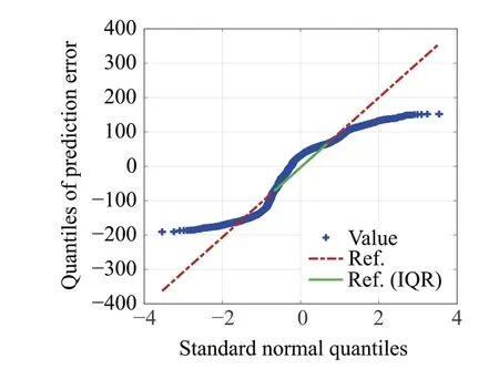
Fig.5 Q-Q plot of road profile(D-E class)

whereΓ= 2k· 10-3，sd∈[0，Lroad]，Δ f= 1/Lroad，nmax=1/fmax，N=nmax/Δn=Lroad/fmax，andfmaxis the highest spatial frequency. The road surface unevenness degree is expressed by thekvalue ofS(f0). The correspondence between thekvalues and the eight road state classifications are listed in Table1. The A and B classes correspond approximately to asphalt，while the D-E classes correspond to irregular roads.The road profile(with respect to the driving distance represented by(16))is shown in Fig.4，whereLroad= 250m， andN= 2500. Increasedkvalues indicate increased vertical height.

Next，we will examine the distribution of road profile characteristics.The D-E class road profile histogram is shown in Fig.6.To compare similarities between normal and sample distributions， the quantile-quantile (Q-Q) plot of the D-E class road profile is shown in Fig.5 where the horizontal axis is the quantiles of the standard normal distribution，and the vertical axis is the sample quantiles. As the quantiles increase in similarity，the tendency of the blue dots to follow the straight line indicated by the red alternating long-short dashed line increases.The green line shows the interquartile.As can be seen in Fig.5，the road profile characteristics differ from the normal distribution.

Fig.6 Histogram of road profile(D-E class)

In this paper，the output is expressed as follows:

whereMkis the Kalman gain， and ˆxk|kandPk|kare the a posteriori state estimate and error covariance，respectively.

This section describes the formulation of the optimization problem designed to achieve vehicle stability. First， we describe the cost function required to balance the input and state priority necessary to achieve the desired performance，after which we describe the constraints. In particular， we examine how uncertainty is considered via the chance constraint in the optimization problem.

5.1 Cost function

In this paper，the evaluation function of the following equation is defined as follows:

5.2 Constraints

Next， we will explain how to transform the chance constraint into a deterministic constraint to solve the stochastic optimization problem as an equivalent deterministic problem

5.3 Optimization problem

Using a vehicle model， a cost function， and the relevant constraints，a deterministic equivalent constrained stochastic programming is expressed as follows:

Fig.7 SMPC system Block diagram

Table 2 Vehicle parameters

In this figure， the black-filled area shows the time evolution after the vehicle has stopped.A comparison between SMPC and MPC model results during braking on a split-μroad with a vertical road profile displacement is shown in Fig.9.The red and blue solid lines show the cases of SMPC and MPC，respectively.The green dashed line shows the ref-erence trajectory.Trajectories on theX-Yplane are shown in Fig.9a，while Fig.9b shows the time evolution of the vehicle longitudinal speed. The lateral deviation time evolution is shown in Fig.9c. The chain line shows constraints. The time evolution of QP iterations is shown in Fig.9d. Here，the yellow line shows that using the QP is infeasible，while the chain line shows max iterations. The time evolution of traveling distance is shown in Fig.9e.The Key Performance Indicators(KPIs)is shown in Table5 and Fig.9f，where index factor is max deceleration， max corrective steering angle，max traveling distance， mean front wheels slip ratio， mean rear wheels slip ratio，max yaw rate[13].The time evolution of execution time is shown in Fig.10，while Fig.10a，c and Fig.10b，d show the SMPC and MPC cases，respectively.The time evolution of brake pressure in the SMPC case is shown in Fig.11， while Fig.11a and b show the SMPC and MPC cases，respectively.Additionally，the slip ratio of each wheel in the SMPC case are shown in Fig.12，while Fig.12a shows the slip ratio of first and second axle wheels.Next，Fig.12b shows the slip ratio of third and fourth axle wheels， while Fig.13 shows the slip ratio of each wheel in the MPC case.

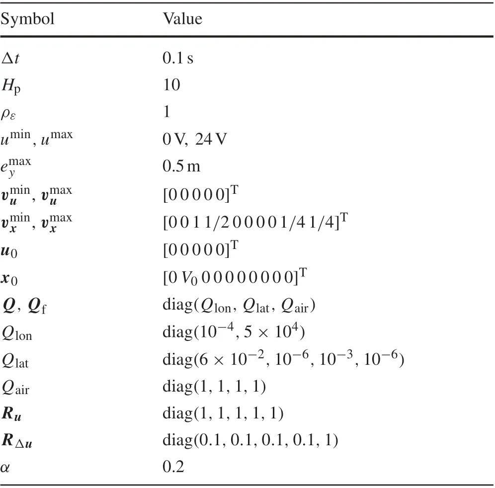
Table 3 Control parameters

Table 4 Estimate parameters

Fig.8 Simulation scenario involving a braking turn on a split-μ road

Fig.9 Comparison between SMPC and MPC during braking on a splitμ road with aa vertical road profile displacement broken down by a trajectory，b longitudinal speed of the vehicle CoG，c lateral deviation，and d quadratic programming (QP) iterations. e Traveling distance. f Key Performance Indicators(KPIs)The red and blue solid lines show the SMPC and MPC cases， respectively， while the green dashed line shows the reference trajectory and the chain lines show constraints.The yellow line shows that using QP is infeasible，while the chain line shows the max iterations

Table 5 KPIs

Fig.10 Execution time.a SMPC(fixed with Δt =100 ms).b MPC(fixed with Δt =100 ms).c SMPC(fixed with Hp =10).d MPC(fixed with Hp =10)

The vehicle braked while maintaining lane tracking in each case，as shown in Fig.9a.As shown in Fig.9c，the lateral deviation constraint was violated in both the SMPC and MPC cases because it was necessary to allow the slack variable constraint to be violated to make the chance constraint of the friction circle feasible.In addition，the lateral deviation in the SMPC case was smaller than in the MPC case because the solution became infeasible in the MPC case when its optimality was lost at the 2-s mark，as shown in Fig.9d.Hence，when considering the statistical information related to disturbances，the results of this study show that lane followability and running stability during braking on a split-μcircular route are improved by the use of SMPC.In Fig.9b，we can see that the SMPC simulation stopping time was slightly longer than the MPC stopping time.However，As shown in Fig.9e， stopping distance of SMPC is 71.8m and MPC is 72.2m. Also， as shown Table5 and in Fig.9f， SMPC KPIs areimprovedcomparedwithMPCKPIs.Theslipratioduring braking in the SMPC case，as shown in Fig.12，was smaller than the MPC case， as shown in Fig.13. This is because SMPC considers the confidence interval of the brake pressure to be a chance constraint and is more conservative than the original constraint， as shown in (31) and Fig.11. As a result，slippage due to uncertainty is suppressed，as shown in Fig.12.In the MPC case，the brake pressure uncertainty is not explicitly considered，so the ratio of time exceeding the tire friction circle constraint is higher than that of SMPC，which means the vehicle slipped more， as shown in Fig.13. The slip ratio values in the black-filled area oscillated after the vehicle stopped as shown in Figs.12 and 13.This is because the formula for calculating the vehicle skid angle has a term that includes velocity in the denominator， and the calculation becomes unstable due to division by zero as the vehicle is braked.From Fig.10，the longer the prediction horizonHpis， the more dimensionality of the matrices handled in the optimization calculation. Therefore， the average and peak execution times are longer.In all cases ofHp=10，7，5，the computation time peaked at 2s，which is the start of stopping，but it was below the sampling time of MPCΔt= 100 ms.This is because the vehicle switched from constant driving，which does not reach the friction circle constraint，to braking，which does reach the friction circle constraint. As a result，the active constraints in the effective constraint method were updated， and the Hesse matrix of the Lagrangian function was re-evaluated. This resulted in a temporary increase in the run time by 2s.

Fig.11 Brake pressure of the front left wheel during braking on the split-μ road with vertical road profile displacement.The green marker shows the measurement values while the red solid line shows the estimation. The blue solid line shows the upper bound predicted by the tire friction circle，while the yellow solid line shows the true value.The violet dashed line shows 2σ confidence interval:a SMPC.b MPC

Fig.12 Slip ratio during braking in a turn on an split-μ road(SMPC).The blackfilled area shows the time evolution after the vehicle has stopped.a First and second left/right wheels，b third and fourth left/right wheels

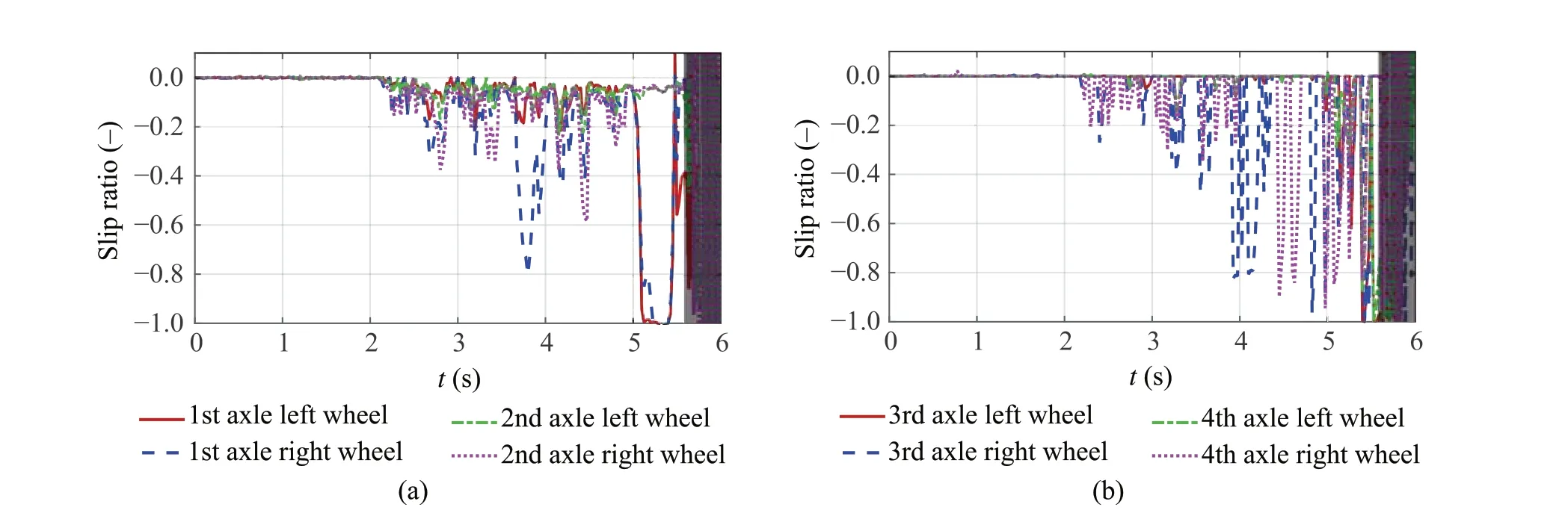
Fig.13 Slip ratio during braking in a turn on an split-μ road(MPC).The black-filled area shows the time evolution after the vehicle has stopped.a First and second left/right wheels，b third and fourth left/right wheels

This paper proposed a method of SMPC that considers the uncertainty of brake pressure and road profiles in relation to the emergency braking of heavy-duty commercial vehicles(HDCVs).Herein，the proposed method was verified through a simulation involving turning braking on a split-μroad.The running stability of an HDCV ensured stable conditions in areas where the controlling braking force and the lateral force interacted.

Open Access This article is licensed under a Creative Commons Attribution 4.0 International License，which permits use，sharing，adaptation， distribution and reproduction in any medium or format， as long as you give appropriate credit to the original author(s) and the source， provide a link to the Creative Commons licence， and indicate if changes were made. The images or other third party material in this article are included in the article’s Creative Commons licence，unless indicated otherwise in a credit line to the material. If material is not included in the article’s Creative Commons licence and your intended use is not permitted by statutory regulation or exceeds the permitteduse，youwillneedtoobtainpermissiondirectlyfromthecopyright holder. To view a copy of this licence， visit http://creativecomm ons.org/licenses/by/4.0/.